The Dirichlet Problem and Continuous Local Martingales
The Dirichlet problem is an important boundary value problem, with applications in physics. Although hard to solve analytically, we can construct probabilistic approximations using continuous local martingales.
In this post, we explore the mathematical connections between the Dirichlet problem and continuous local martingales, and compute an example using Python. The source code is available on GitHub.
The Dirichlet problem
To solve the Dirichlet problem on a region, we must find a function that:
- satisfies a certain PDE in the region
- satisfies a given boundary condition at the boundary of the region
The PDE determines how the function “behaves” inside the region, while the boundary condition “constrains” it at the edges. We make these notions rigorous below.
Mathematical formulation
Let $U \subseteq \mathbb{R}^d$ be an open bounded connected set,
with closure $\bar{U}$ and boundary $\partial U$.
Let $f: \bar{U} \to \mathbb{R}$ be twice continuously
differentiable $(\mathcal{C}^2)$ on $U$,
and continuous on $\bar{U}$.
Let $\phi: \partial U \to \mathbb{R}$ be continuous.
We say $f$ solves the Dirichlet problem on $U$ with boundary condition $\phi$ if
- $\nabla^2 f = 0\ $ on $\ U$
- $f = \phi\ $ on $\ \partial U$
Recall that the Laplace operator is defined by
\[\nabla^2 = \nabla \cdot \nabla = \sum_{i=1}^d \frac{\partial^2}{\partial x_i^2}\]Comments
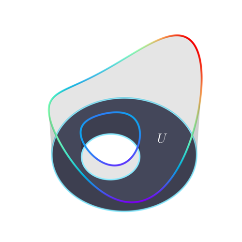
A solution to the Dirichlet problem in two dimensions can be visualised by drawing the region $U$ on the ground, and suspending a loop of wire over its boundary $\partial U$, where the height of the wire corresponds to the value of $\phi$. Then attach a taut rubber sheet to this wire, above the region. The solution $f$ is given by the height of this sheet at each point. In other words, the Dirichlet problem corresponds in some sense to finding the surface with least energy, which equals $\phi$ on the boundary.
This same intuition applies to the electrical field inside a hollow charged shell, albeit this time in three dimensions.
Note that the Dirichlet problem is a deterministic boundary value problem (at least when unique solutions exist), and does not explicitly concern probability at all. This makes the connection with stochastic processes all the more surprising!
Continuous local martingales
Continuous local martingales are a special type of stochastic process. They are generalisations of continuous martingales, and exhibit deep connections with second-order PDEs.
Definition
Let $\big(\Omega, \mathcal{F}, (\mathcal{F}_ t), \mathbb{P}\big)$ be a complete filtered probability space. We say that a continuous adapted process $(X_ t)$ is an $(\mathcal{F}_ t)$-continuous local martingale if we can find a sequence of $(\mathcal{F}_ t)$-stopping times $(\tau_ k)$ such that
- $(\tau_k)$ is a.s. increasing
- $(\tau_k)$ a.s. diverges to $\infty$
- $X_ {t \wedge \tau_k}$ is an $(\mathcal{F}_ t)$-martingale for each $k$
The sequence $(\tau_ k)$ is called a localising sequence.
Properties of continuous local martingales
We will need to use two properties of continuous local martingales. The first is a simple extension of Doob’s optional stopping theorem for martingales. The second is a property of stochastic integration, in which continuous local martingales play a central role.
Proposition 1 (optional stopping theorem)
Let $(X_ t)$ be a bounded continuous local martingale, and $\tau$ an a.s. finite stopping time. Then
\[\mathbb{E}[X_\tau] = \mathbb{E}[X_0]\]Proof
Let $(\tau_ k)$ be a localising sequence for $(X_ t)$, and $s \leq t$. Since $(X_ t)$ is continuous and bounded, the conditional dominated convergence theorem (DCT) gives
\[\begin{align*} \mathbb{E}[X_ \tau] &= \mathbb{E}[\lim_ {k \to \infty }X_ {\tau \wedge \tau_ k}] &\text{(as } \tau_ k \to \infty \text{)} \\ &= \lim_ {k \to \infty }\mathbb{E}[X_ {\tau \wedge \tau_ k}] &\text{(conditional DCT)} \\ &= \lim_ {k \to \infty }\mathbb{E}[\lim_ {t \to \infty} X_ {\tau \wedge \tau_ k \wedge t}] &\text{(as } \tau < \infty \text{)} \\ &= \lim_ {k \to \infty }\lim_ {t \to \infty} \mathbb{E}[X_ {\tau \wedge \tau_ k \wedge t}] &\text{(conditional DCT)} \\ &= \mathbb{E}[X_0] &\qquad \text{(as } (X_ {t \wedge \tau_ k}) \text{ is a martingale)} \\ \end{align*}\]Proposition 2 (stochastic integrals as local martingales)
Let $B_ t$ be a Brownian motion with canonical filtration $(\mathcal{F}_ t)$. Let $X_ t$ be a bounded process adapted to $\mathcal{F}_ t$. Then the stochastic integral
\[Y_ t = \int_0^t X_ s \d B_ s\]defines a process $(Y_ t)$ which is a local martingale. We sometimes for brevity write
\[\d Y_ t = X_ t \d B_ t\]Proof
The proof is technical but is a standard result in stochastic analysis.
The Itô formula
The Itô formula serves as a “chain rule” for stochastic calculus. Here we state a special form of it, for integrals against Brownian motion.
Proposition 3 (Itô formula)
Let $\big(\Omega, \mathcal{F}, (\mathcal{F}_ t), \mathbb{P}\big)$
be a complete filtered probability space,
which carries a $d$-dimensional Brownian motion
$(B_ t) = (B^1_ t, \ldots B^d_ t)$.
Let $f: \mathbb{R}^d \to \mathbb{R}$
be in $\mathcal{C}^2$.
Then
Hence by Proposition 2, $f(B_ t)$ is the sum of a local martingale term and a regular Stieltjes integral against$\d t$.
The link between continuous local martingales and the Dirichlet problem
Take $U$ a region as before, and suppose $f$ solves the Dirichlet problem in $U$ with boundary condition $\phi$.
For each $x \in U$, let $B^x$ be a $d$-dimensional Brownian motion started from $x$. Let
\[\tau_ x = \inf \{ t \geq 0 : B^x_ t \not\in U \}\]be the escape time of $B^x$ from $U$. It is a stopping time because it is the first hitting time of a closed set by a continuous adapted process. Consider the process given by
\[(X^x_ t) = f(B^x_ {t \wedge \tau_ x})\]Proposition 4
$(X^x_ t)$ is a continuous local martingale on $[0, \tau_ x)$.
Proof
By the Itô formula, for $0 \leq t < \tau_ x$
\[\begin{align*} \d X^x_ t &= \d f(B^x_ t) \\ &= \nabla f(B_ t)^\mathsf{T} \d B_ t + \frac{1}{2} \nabla^2 f(B_ t) \d t \\ &= \nabla f(B_ t)^\mathsf{T} \d B_ t \end{align*}\]since $\nabla^2 f = 0$ in $U$. So $X^x_ t$ is a stochastic integral against a Brownian motion, and forms a continuous local martingale, by Proposition 2.
Proposition 5
For all $x \in U$, we have $\mathbb{E}[\phi(B^x_ {\tau_ x})] = f(x)$
Proof
Firstly, the left hand side makes sense because a.s. $B^x_ {\tau_ x} \in \partial U$. Now since $U$ is bounded, it is a basic fact about Brownian motion that $\tau_ x$ is a.s. finite. Further, $f$ is a continuous function on a compact set, so $(X^x_ t)$ is bounded. Hence by the optional stopping theorem:
\[\begin{align*} \mathbb{E}[\phi(B^x_ {\tau_ x})] &= \mathbb{E}[f(B^x_ {\tau_ x})] &(f = \phi \ \text{ on }\ \partial U) \\ &= \mathbb{E}[X^x_ {\tau_ x}] \\ &= \mathbb{E}[X^x_ 0] \\ &= \mathbb{E}[f(B^x_ 0)] \\ &= \mathbb{E}[f(x)] \\ &= f(x) \end{align*}\]Approximate constructive solutions
The above propositions prove that if a solution exists to the Dirichlet problem in $U$ with boundary condition $\phi$, then it is uniquely determined. Moreover, they suggest a constructive method to approximate the solution $f$, using Monte Carlo simulation:
\[f(x) = \mathbb{E}[\phi(B^x_ {\tau_ x})] \approx \frac{1}{M} \sum_ {m=1}^M \phi\big(B^{x,m}_ {\tau_ {x,m}}\big)\]by the strong law of large numbers, where $M$ is large and $\{B^{x,m}\}_ {m=1}^M$ are independent Brownian motions started from $x$.
An example
To illustrate this method, we compute an approximate solution to a Dirichlet problem in two dimensions.
Problem data
First we choose a suitable region $U$:
$U = A \setminus B$ where $A$ and $B$ are the nested discs
\[\begin{align*} A &= \{(x,y) : (x-1)^2 + y^2 < 5^2\} \\ B &= \{(x,y) : x^2 + y^2 < 2^2\} \end{align*}\]The boundary condition $\phi$ defined on $\partial U$ is
\[\phi(x,y) = x^2 + y + 10 \\\]
Simulating Brownian motion
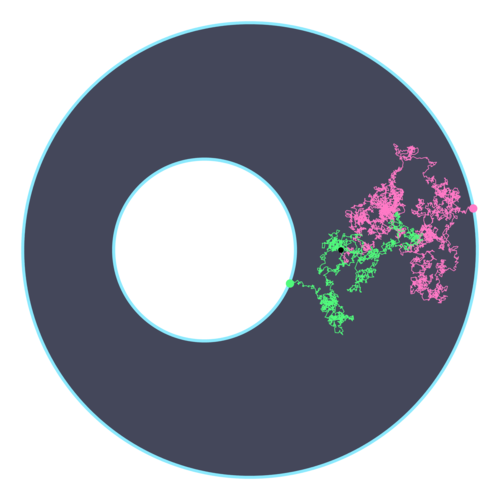
Since Brownian motion is a complex object, it is not possible to simulate it exactly. Instead we use a discrete-time process $\beta^{x,\delta}$ defined by
\[\beta^{x,\delta}_ n = x + \sum_ {i=1}^n \frac{Z^{x,\delta}_i}{\sqrt{\delta}}\]where $Z^{x,\delta}_ i$ are independent standard Gaussian random variables. Note that $\beta^{x,\delta}$ satisfies
\[\big(\beta^{x,\delta}_ 1, \ldots, \beta^{x,\delta}_ n\big) \sim \big(B^x_ \delta, \ldots, B^x_ {n\delta}\big)\]where $\sim$ indicates equal distributions. With a sufficiently small time step $\delta$, this is a useful approximation to Brownian motion. It is also easy to find the first escape time of $\beta^{x,\delta}$ from $U$, and to stop the process at that time.
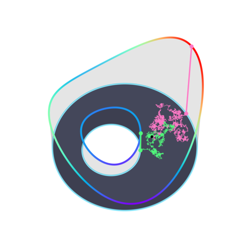
Figure 3 plots two sample paths of the approximate Brownian motion started from the same point, up to their respective escape times. Figure 4 also shows the boundary values $\phi$ at the escape times. The time step used was $\delta = 0.001$.
Results
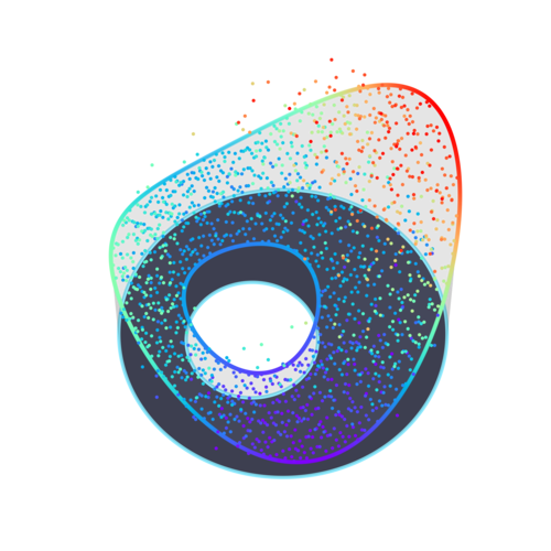
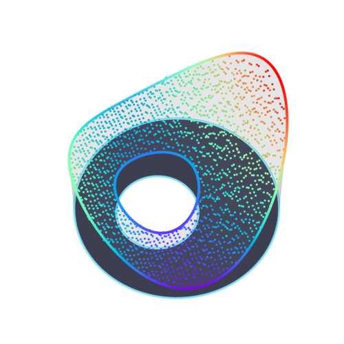
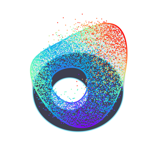
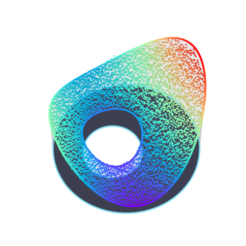
We take a square grid of starting points $x \in U$, with distance $\epsilon$ between neighbouring points. Then approximate Brownian motions with time step $\delta = 0.001$, started from $x$, are simulated up to their escape times. This is repeated $M$ times, and the Monte Carlo estimate is computed separately for each $x$.
Figures 5–8 show how decreasing $\epsilon$ improves the spatial fidelity of the estimate, while increasing $M$ reduces the variance. The “rubber sheet” analogy is very clear, especially in the last plot, as the estimates converge towards a surface of least energy.
Comments
This method for solving PDEs by constructing a suitable continuous local martingale is by no means restricted to the Dirichlet problem. The Feynman–Kac formula provides a more general method for solving second-order PDEs, by employing slightly more complex stochastic processes.
These results hint at some of the deep connections between PDEs and stochastic processes, in particular what is known as the generator of a Markov process. In the case of Brownian motion, this generator is $\frac{1}{2} \nabla^2$, the same operator which is seen in the Dirichlet problem. Other stochastic processes have different generators, and so can be used to construct solutions to different PDEs.
References
- The Wikipedia page on the Feynman–Kac formula
- The Wikipedia page on stochastic processes and boundary value problems
- This blog post on Eventually Almost Everywhere